Fiting a SED

import matplotlib.pyplot as plt
import torch
import sedpy
import starduster
from scipy.optimize import minimize

torch.set_num_threads(1)
torch.manual_seed(999);

This tutorial demonstrates how to fit a SED. We start by building the SED model.

sed_model = starduster.MultiwavelengthSED.from_builtin()
sed_model.configure(
    pn_gp=starduster.GalaxyParameter(),
    pn_sfh_disk=starduster.CompositeGrid(
        starduster.InterpolatedSFH(), starduster.InterpolatedMH(),
    ),
    pn_sfh_bulge=starduster.CompositeGrid(
        starduster.InterpolatedSFH(), starduster.InterpolatedMH(),
    ),
    flat_input=True,
)

We then create some mock photometric data. The easiest way to ouput filter fluxes is to use the transmission curves given by sedpy.

band_names = [
    'galex_FUV', 'galex_NUV',
    'sdss_u0', 'sdss_g0', 'sdss_r0', 'sdss_i0', 'sdss_z0',
    'twomass_J', 'twomass_H', 'twomass_Ks',
    'wise_w1', 'wise_w2', 'wise_w3', 'wise_w4',
    'herschel_pacs_100', 'herschel_pacs_160',
    'herschel_spire_250', 'herschel_spire_350', 'herschel_spire_500'
]
filters = sedpy.observate.load_filters(band_names)
redshift = 0.01
distmod= 0.
sed_model.configure(filters=filters, redshift=redshift, distmod=distmod, ab_mag=True)
# Generate a random SED
params_true = starduster.sample_effective_region(sed_model)
with torch.no_grad():
    mags = sed_model(params_true, return_ph=True)
# We assume 0.1 mag error for every band
mags_err = torch.full_like(mags, 0.1)

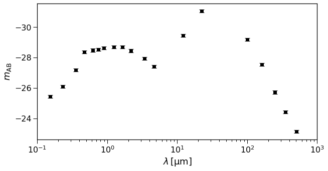
The figure below shows the mock SED.

fig, ax = plt.subplots(figsize=(10, 5))

lam_pivot = sed_model.lam_pivot.numpy()
plt.errorbar(lam_pivot, mags.numpy(), mags_err.numpy(), fmt='ks')

ax.set_xscale('log')
ax.set_xlabel(r'$\lambda \, [\rm \mu m]$')
ax.set_ylabel(r'$m_{\rm AB}$')
ax.set_xlim(.1, 1e3)
ax.invert_yaxis()

This next step is to build the posterior distribution. Posterior is callable, which provides a good interface for various optimisers and sampling tools.

noise_model = starduster.IndependentNormal(mags, mags_err)
# Create the initial value for the optimiser
eps = 0.1
sampler = lambda n_samp: params_true + eps*(2*torch.rand(n_samp, len(params_true)) - 1)
params_0 = starduster.sample_effective_region(sed_model, sampler=sampler)

The following code uses the Adam optimiser given by PyTorch to fit the SED. This optimiser requires the first-order gradient.

posterior = starduster.create_posterior(sed_model, noise_model, mode='torch', negative=True)
params_pred = starduster.optimize(
    posterior, torch.optim.Adam, params_0, n_step=300, lr=1e-2
)

loss: -2.628e+01: 100%|██████████| 300/300 [00:06<00:00, 44.79it/s]

We may also use the Scipy LBFGS optimiser. We can pass the first-order gradient by setting jac=True.

posterior = starduster.create_posterior(sed_model, noise_model, mode='numpy_grad', negative=True)
res_bfgs = minimize(
    posterior, params_0.numpy(), bounds=sed_model.bounds, method='L-BFGS-B', jac=True
)
params_bfgs = res_bfgs.x

Additonaly, we can also employ a optimiser that does not require the gradient. The following output mode can also be applied to a MCMC sampler.

posterior = starduster.create_posterior(sed_model, noise_model, mode='numpy', negative=True)
res_powell = minimize(
    posterior, params_0.numpy(), bounds=sed_model.bounds, method='Powell'
)
params_powell = res_powell.x

We compare the results obtained by different optimisers as follows. The results are consistent.

print("\tTrue\tAdam\tLBFGS\tPowell")
for params in zip(params_true, params_pred, params_bfgs, params_powell):
    print("\t%.2f\t%.2f\t%.2f\t%.2f"%params)

        True    Adam    LBFGS   Powell
        0.60    0.69    0.70    0.70
        0.27    0.31    0.28    0.31
        -0.16   -0.24   -0.17   -0.24
        -0.14   -0.14   -0.14   -0.14
        -0.39   -0.38   -0.39   -0.38
        0.86    0.86    0.86    0.86
        -0.93   -0.93   -0.92   -0.93
        8.44    8.44    8.44    8.44
        0.04    0.06    0.06    0.06
        8.15    8.12    8.12    8.12
        0.00    -0.12   -0.12   -0.13

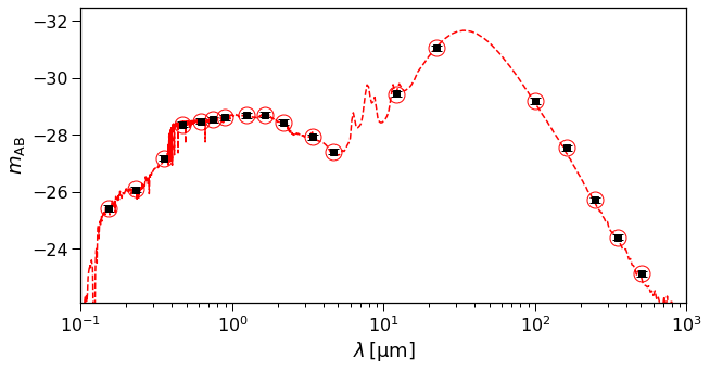
The fitting result can be seen in the figure below.

# Compute the fitting result
with torch.no_grad():
    f_nu = sed_model(params_pred)
    f_ab = -2.5*torch.log10(f_nu) + 8.9
    mags_pred = sed_model(params_pred, return_ph=True)

# Plot the result
fig, ax = plt.subplots(figsize=(10, 5))

plt.errorbar(lam_pivot, mags, mags_err.numpy(), fmt='ks')
plt.plot(lam_pivot, mags_pred, 'ro', markersize=15, markerfacecolor='none')
plt.plot(sed_model.lam, f_ab, 'r--')

ax.set_xscale('log')
ax.set_xlabel(r'$\lambda \, [\rm \mu m]$')
ax.set_ylabel(r'$m_{\rm AB}$')
ax.set_xlim(.1, 1e3)
ax.set_ylim(top=mags.numpy().max() + 1)
ax.invert_yaxis()